Data Analysis and Statistics Study Guide for the Math Basics

Calculating Rate

Rate or Rate of change is the ratio of how much one one quantity changes per unit of another. Common rates you might be familiar with: speed (miles per hour, kilometers per hour, feet per second, etc.), heart rate (beats per minute) and fuel efficiency (miles per gallon), to name a few.

For instance, if you are driving at a speed of 60 mph, then that means you travel 60 miles in one hour.

To calculate the rate, simply divide one quantity by the other. Remember, the word per means division. If your heart beats 328 times in a 4 minute interval, then:

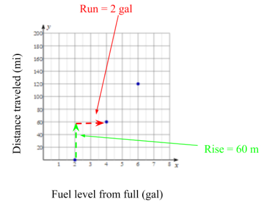
\[heart \; rate = \dfrac{328 \; beats}{4 \;minutes} = \dfrac {82 \; beats}{1\;minute} = 82 \;bpm\]

For bivariate data (comparing two variables), rate is commonly referred to as the slope of the graph. Take the following graph comparing distance travelled and fuel used.

The ordered pairs on the graph are: \((2,0), (4,60),\; and \;(6,120)\)

Here are some common ways to represent the rate of change, or slope using this example.

\[rate\;of\;change=\dfrac{rise}{run}\]

You can do this using any two points provide the data is linear.

\[rate \; of \; change = \dfrac{rise}{run}=\dfrac{60 \;m}{2\; gal}= 30 \;mpg\]

Another way to calculate the rate of change is the following formula:

\[rate \; of \; change = \dfrac{y_2-y_1}{x_2-x_1}\]

Use any two points for \((x_1, y_1), (x_2, y_2)\). In this case, let’s use \((x_1, y_1)=(2,0)\) and \((x_2, y_2)=(6,120)\). So:

\[rate \; of \; change = \dfrac{120-0}{6-2}=\dfrac{120}{4} = 30 \;mpg\]

Data Concepts

Once a graph or chart is made from the data, we can start analyzing the data using some of these concepts.

Line of Best Fit

You find the line of best fit of a scatterplot. Most database programs or your graphing calculator can find them, which is usually the best option because the math is quite advanced. However, you can always try to draw a line that you think represents the data, and calculate its slope and y-intercept to find the line of best fit. Here’s an example from the scatterplot above.

Correlations

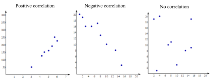
When looking at a scatterplot, you should immediately be able to determine if it has a positive correlation, negative correlation or no correlation.

If the data has positive correlation, the best fit line would have a positive slope (going up and to the right) just like the example above.

If the data has negative correlation, the best fit line would have a negative slope (going down and to the right).

If it looks like the data is not really trending in any direction, we say there is no correlation.

Distributions

There are two main kinds of distributions you’d come across: normal and random.

In general, a set of data has a normal distribution if more values fall in the middle of the data than at the extremes.

Here’s an example of a normally distributed data set.

A set of data has a random distribution if it seems that no section of the data is more concentrated than the rest.

Standard Deviation

The standard deviation, often represented by the greek letter sigma (\(\sigma\)), is a measure of how spread out the data is. To calculate the standard deviation, follow these steps with this example.

\[\{5, \; 7, \; 12, \; 8, \; 10, \; 6\}\]

1) Find the mean:

\[\dfrac{5+7+12+8+10+6}{6}=\frac{48}{6}=8\]

2) Find the differences of each value from the mean and make a set of them.

\[8-5=3,\; 8-7=1, \;12-8=4, \;8-8=0, \;10-8=2,\; and \; 8-6=2\] \[Differences = \{3, \; 1, \; 4, \; 0, \; 2, \; 2\}\]

3) Now square the differences.

\[Squares \; of \; differences = \{3^2, \; 1^2, \; 4^2, \; 0^2, \; 2^2, \; 2^2\}\] \[Squares \; of \; differences = \{9, \; 1, \; 16, \; 0, \; 4, \; 4\}\]

4) Find the average of these. This value is called the variance.

\[Variance = \dfrac{9+1+16+0+4+4}{6}=\dfrac{34}{6}= 5 \frac{2}{3}\]

5) Finally, the standard deviation is the square root of the variance.

\[\sigma=\sqrt{variance}=\sqrt{5 \frac{2}{3}} \approx 2.38\]

Outliers

In general, outliers are data points that are isolated from the rest of the data. Statistically, a test might define outliers to be data points that are more than 3 standard deviations from the mean.

In the previous example, the mean is \(8\) and \(\sigma=2.38\). So, \(3\sigma=7.14\). Therefore, any outliers would fall below \(0.86\) (\(8-7.14\)) or above \(15.14\) (\(8+7.14\)). No values do, so there were no outliers.

Interpretations and Predictions

Often, tests will ask you to make predictions based on a given data set. Let’s look at the following example and make and interpolation and extrapolation.

A linear interpolation is an estimation of a value between given data points. You can interpolate that the savings balance in April will be somewhere between the values of March ($75) and May ($85). A pretty good guess would be that the savings balance in April will be $80.

To extrapolate information means to make an estimation of a value outside of the data set. For instance, we can extrapolate what the balance might be the following January (two months after November). It looks like the balance goes up $10 to $20 every two months, so we’d guess that the value next January would be between $150 and $160. A good guess would be $155.

Probability

As we’ve already seen, we look at past events to predict what might happen next. One valuable way to do this is by using probability or the likelihood that something might occur given conditions are similar to what has been observed.

\[Probability=\dfrac{\text{number of past successes}}{\text{total number of past outcomes}}\]

Let’s say a baseball player has had 120 at bats up to this point in the season. If he’s gotten on base 45 times in those at bats, what’s the likelihood he gets on base next at bat?

\[Probability=\dfrac{45}{120}=0.375=37.5\%\]

Of course, sometimes probability isn’t based on past observations, but merely looking at the amount of ways something could happen. Take a dice roll for example. What’s the probability of rolling an even number? Let’s use the following definition of probability:

\[Probability=\dfrac{\text{number of ways to succeed}}{\text{total number of possible outcomes}}\]

In this case, we can succeed if we roll a 2, 4, or a 6 (there are three ways). There are 6 total number of ways to roll a dice, so:

\[Probability = \dfrac{3}{6} = 0.5 = 50\%\]