Basic Algebra Study Guide for the Math Basics

Algebra and Graphing

A large section of algebra focuses on bivariate data, how one variable changes based on another variable. One of the best ways to represent those relationships is on a coordinate plane: a two dimensional flat space where two number lines intersect perpendicularly at \(0\), or the origin. These two number lines are called the x and y axes. The plane is split into four quadrants, where quadrant 1 is the upper right quadrant and they count up going in a counterclockwise direction. A point on the plane is denoted by an ordered pair representing its x-coordinate and its y-coordinate. Here’s a coordinate plane with the quadrants labeled and the point \((3,-5)\) represented as a blue dot.

Slope

In Algebra I, you’ll usually be investigating linear data almost exclusively. That means that, as one variable changes, the other one changes at a constant rate. This rate is called the slope of the line. There is a formula to find the slope between any two points \((x_1, y_1)\) and \((x_2,y_2)\) on the line.

\[\text{slope} = \dfrac{y_2\;-\;y_1}{x_2\;-\;x_1}\]

Graphically, you might find the slope this way:

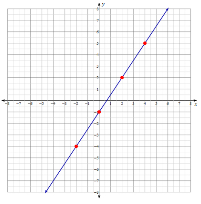
\[\text{slope} = \dfrac{\text{rise}}{\text{run}}\]

Let’s examine this line, with certain points on the line shown in red.

There are four points: \((-2,-4), \; (0, -1), \; (2, 2), \; \text{and } (4,5)\) which fall exactly on lattice points (integer amounts), among others.

Choose any two points and algebraically find the slope. Let’s let \((x_1, y_1) = (-2,-4)\) and \((x_2,y_2) =(2,2)\).

\[\text{slope} = \dfrac{2-(-4)}{2-(-2)}\] \[\text{slope} = \dfrac{6}{4}\] \[\text{slope} = \dfrac{3}{2}\]

It does not matter which two points we choose. Let’s use the \(\dfrac{\text{rise}}{\text{run}}\) method between two other points on the line.

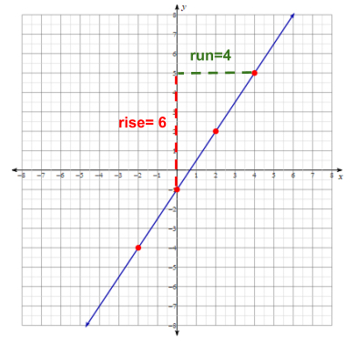
So, the slope between \((0,-1)\) and \((4,5)\) is:

\[\text{slope}=\dfrac{\text{rise}}{\text{run}}=\dfrac{6}{4}=\dfrac{3}{2}\]

This is exactly what we obtained using the algebraic method.

Intercept

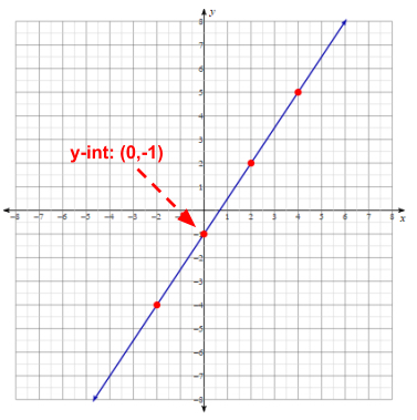
Aside from slope, another important feature of the line is its y-intercept: where the line crosses the x-axis. Sometimes it’s straightforward and you can see it exactly on the graph, like in the line we’ve already been examining.

Occasionally, the y-intercept doesn’t land directly on an integer amount. In this case, you’ll have to use the equation of the line and substitute \(0\) in for x, because \(x=0\) everywhere on the y-axis. Or maybe you’ll have to manipulate a different form of an equation into slope-intercept form. See an example of this in the examples section of using formulas.

Linear Forms

There are three main forms we use to write the equation of a line.

The most common form is slope-intercept form. In this case, let m = the slope of the line, b = the y-intercept, and x and y will represent any point on the line. The equation is:

\[y=mx+b\]

Occasionally we might use the point-slope form of the line. Let m = the slope of the line again, \((x_1, y_1)=\) a known point on the line, and x and y again represent any other point on the line. This equation is:

\[y-y_1=m(x-x_1)\]

One more form we use, usually when x and y intercepts are known, is the standard form. This represents the relationship between the x and y variables of any point on the line using the equation:

\[Ax+By=C\]

Note: A, B, and C must all be integers, with no common factors other than 1.

Using Formulas

There are many mathematical relationships which we know and we represent them as a formula. Formulas use variables and numbers and are used when we only know certain parts of the relationship, but we wish to know the rest. For example, I might know the radius of a circle, but I want to know the area. There’s a formula for that. Or maybe I’ve been traveling for some time at a certain speed and I want to know how far I’ve gone. There’s a formula for that, too.

Substitution Property

At the core of using formulas is the substitution property which states that if \(a=b\), then a may be replaced by b in any expression. For example, If \(a=b\) and an expression says that \(a+5=9\), then \(b+5=9\) is also true.

Examples

Here’s a common word problem you might encounter: I drove from St. Louis to Kansas City in 4 hours. If the distance between the two cities is 250 miles, what was my average speed?

For this problem, the question is “what was my average speed?”. Let s=average speed. Other useful information is that time = 4 hours and distance = 250 miles. Now, use the distance formula, substitute, and solve.

\[\require{cancel}\] \[\text{distance}= \text{speed } \cdot \text{ time}\] \[250 \text{ miles}= s \cdot 4 \text{ hours}\] \[250 \text{ miles} \div 4 \text{ hours} = s \cdot \cancel{4 \text{ hours}} \div \cancel{4 \text{ hours}}\] \[62.5 \text{ mph}= s\]

Now, let’s see an algebraic problem. Suppose you want to find the y-intercept of a line with slope \(=\dfrac{3}{2}\) that passes through the point \((x_1,y_1)=(5,3)\). Clearly, since you’re given the slope and a point, you’ll want to substitute these values into the point-slope form:

\[y-y_1=m(x-x_1)\] \[y-3=\dfrac{3}{2}(x-5)\]

But you don’t know the y-intercept unless the equation is in slope-intercept form: \(y=mx+b\). So, you should distribute and then isolate y.

\[y-3=\dfrac{3}{2}x-7.5\] \[y-3+3=\dfrac{3}{2}x-7.5+3\] \[y=\dfrac{3}{2}x -4.5\]

In this form, it’s easy to see that the slope is \(m=\frac{3}{2}\) and the y-intercept is \(b=-4.5\).

Formulas are used very commonly in geometry. You probably already know that the formula for the area of a circle is \(A=\pi r^2\), where \(\pi \approx 3.14\). So, now, find the area of a circle that has a radius of 9 centimeters. \(r=9\), so substitute \(9\) for \(r\) in the equation.

\[A=\pi r^2\] \[A= \pi \cdot 9^2\] \[A=\pi \cdot 81\]

which can be rewritten as the exact answer:

\[A= 81 \pi \text{ cm}^2\]

But, you can now approximate the answer using \(\pi = 3.14\)

\[A \approx 81 \cdot 3.14 \text{ cm}^2\] \[A \approx 254.34 \text{ cm}^2\]