Math Study Guide for the SAT Exam
Page 1
General Information
There are two timed sections of the SAT exam Math section: one during which you may use a calculator and the other during which you may not. The calculator-allowed section contains 38 questions, and you will be given 55 minutes to complete them. There are 20 questions in the no-calculator section, which is timed for 25 minutes. There is more information on calculator use in the SAT’s Calculator Policy.
Math Skill Areas Assessed
Within both of these sections are questions pertaining to the following four areas of math. For study time allocation purposes, we show the number of questions posed on each topic:
-
Heart of Algebra—19
-
Problem Solving and Data Analysis—17
-
Passport to Advanced Math—16
-
Additional Topics—6
Question Types
Most of the questions in both sections are standard multiple-choice, but you will also encounter a few questions that require you to “grid in” your answer. This means that there will not be answers to choose from. You must arrive at the answer and write or type it in the boxes provided. By section, the numbers of grid-in questions are:
Calculator Section—8
No-Calculator Section—5
See these gridding-in guidelines for more information.
Below is a complete review of the skills covered for each of these topics.
Provided References
During the test, you will have access to this reference, but be sure to be familiar with how and when to use each of them when answering questions.
Heart of Algebra
One of the four types of questions on the SAT exam, Math section, involves dealing with algebra concepts. These questions will test your understanding of, and ability to use linear equations, systems of these equations, and inequalities. Just what do you need to know?
First, you need to be extremely familiar with the terms used in algebra so they don’t trip you up or cause you to spend extra time dissecting a question. Be sure to have a full understanding of all of these and anything else you encounter while studying for this type of question.
Variable vs. Constant
A variable, often designated with a letter (\(x\), \(y\), or \(z\), for example) is used to represent an unknown quantity that may change its value over the course of a problem.
A constant, on the other hand, is a value that does not change, regardless of the circumstances.
Consider the following situation: John is paid a weekly base wage of \(\$15\). In addition to this base wage, he earns \(\$0.25\) for every magazine he sells. Write an equation representing John’s total wage.
In this case, the base wage John earns is a constant, so regardless of the number of magazines he sells, he will gain \(\$15\). If he sells \(0\) magazines, he will earn \(\$15\). If he sells \(1\) magazine, he will earn \(\$15 + \$0.25, or \$15.25\). We can use a variable to represent the unknown number of magazines he sells and combine this with his base wage to express his total wage. Let \(m\) represent the unknown number of magazines sold, and let \(f(m)\) be his total wage:
\[f(m) = 0.25 \cdot m + 15\]Because he earns \(\$0.25\) per magazine sold, when we find the product of this with the number of magazines sold, \(m\), we are finding the total amount of money earned from the magazines he has sold. By combining this with his base wage, we calculate his total wage.
Coordinate Plane
The coordinate plane provides a two-dimensional space with which to graphically represent points, lines, and functions in two or fewer variables; it is also known as the \(xy\)-axis. The horizontal axis is the \(x\)-axis, and the vertical axis is the \(y\)-axis. The origin is the intersection of the \(x\)-axis and the \(y\)-axis and is located at point \((0,0)\). This intersection creates four quadrants:
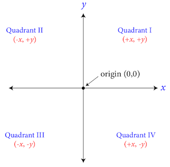
These four quadrants begin with the top right as quadrant I. The quadrants increase in number in a counterclockwise fashion. The quadrant to the left of quadrant I is designated quadrant II. The quadrant below quadrant II is quadrant III, and the remaining quadrant is quadrant IV.
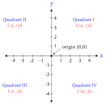
Quadrant I contains positive \(x\) and positive \(y\) values.
Quadrant II contains negative \(x\) and positive \(y\) values.
Quadrant III contains negative \(x\) and negative \(y\) values.
Quadrant IV contains positive \(x\) and negative \(y\) values.
The coordinate plane is most useful for showing the relationship between two variables. The \(x\) variable is commonly referred to as the independent variable (meaning the value of the variable is chosen), and the \(y\) variable is commonly referred to as the dependent variable (meaning its value is determined by the function containing the independent variable).
Points, given in the form \((x,y)\), are commonly graphed on the coordinate plane. The point \((-3,2)\), for example, would be located three units to the left of the origin \((0,0)\), and two units above the \(x\)-axis.
Functions of the form \(f(x) =\) can be graphed in the coordinate plane by selecting values for \(x\), determining their corresponding y values, and then placing points at each of the calculated \((x,y)\) values. The nature of the function determines whether a straight or curved line can be drawn to connect each of the points.
Graph Concepts: Slope and Intercept
The slope of a line is the ratio of the change in \(y\) values to the change in \(x\) values:
\[m = \frac{y_2 - y_1}{x_2 - x_1}\]where
\((x_1, y_1)\) and \((x_2, y_2)\)
are points on the line.
It is helpful to think of the slope as the rise over the run, but it is also important to understand that a line is straight because the change in the \(y\) values is in proportion with the change in the \(x\) values. If this was not so, the graph would exhibit a different characteristic.
Aside from the slope, graphs of lines will also exhibit \(x\) or \(y\)-intercepts. These are points at which lines cross the \(x\) or \(y\) axis. These points are important because they show the \(x\) value of the function when \(y\) is equal to \(0\), and the \(y\) value of the function when \(x\) is equal to \(0\).
Linear Equation vs. Linear Expression
The fundamental difference between an equation and an expression is that an equation contains two expressions that are equal to each other. This equality is represented with the equal sign, \(=\).
Expressions cannot be solved. Instead, where possible, they can be simplified, or reduced. Consider the following expression:
\[4x - 2x + 3x^2 + 5x^2\]The terms containing the same variable type can be combined and the expression can be simplified:
\[4x - 2x = 2x\]and
\[3x^2 + 5x^2 = 8x^2\]so the expression can be rewritten as:
\[2x + 8x^2\]Remember that only like terms can be combined. \(2x\) and \(2x^2\) cannot be combined because the variable is to a different degree.
A linear equation containing one variable can be numerically solved for the variable. A linear equation containing two or more variables can only be solved in terms of those variables. For example:
\[2y + 3x - z = 10\]We can solve this equation for \(x\), \(y\) or \(z\), but the other side of the equation will still contain the other two variables. To solve for all three variables, we must have at least three distinct equations.
Linear Inequality
A linear inequality compares \(x\) and \(y\) expressions using \(\gt, \;\ge, \;\lt,\) or \(\le\). Linear inequalities are simplified in the same way that linear equations are simplified, with one major difference. When a linear inequality is multiplied or divided by a negative integer, the direction of the inequality sign switches, for example:
\(-4x < 8\)
\(x > -2\)
Graphing Inequalities
Inequalities containing an equal sign are graphed differently than those without it.
Consider the following situations:
\[y > x\]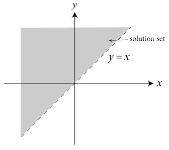
This graphs as an upward-sloping, dotted line. The solution set is every point above the line, not including the points lying along the line.
\[y < x\]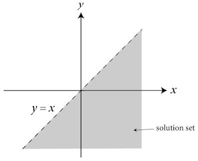
This equation graphs similarly, except the solution set is every point below the dotted line, not including the points lying along the line.
\[y >= x\]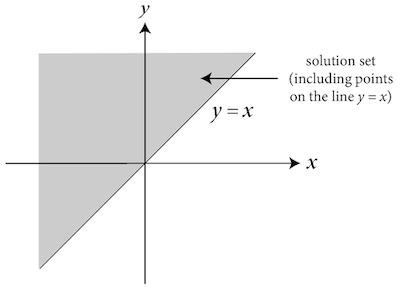
This one graphs like the first, except instead of a dotted line, a bold line is used. This indicates that the points lying along the line are part of the solution set.
\[y <= x\]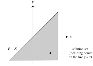
This graph includes a bold line and the area below it is shaded to indicate that every point on and below the line is part of the solution set.
Rational Coefficient
Rational coefficient is a term for any number that is the ratio of two integers with the denominator of the ratio not equalling \(0\).
\(2, \frac{0}{1}, \frac{1}{25}\), and \(\sqrt{25}\) are all rational coefficients.
\(\frac{3}{0}\) and \(\sqrt{2}\) are not considered rational coefficients; the first is undefined, and the second cannot be represented as the fraction of two integers.
Interpret, Simplify, and Solve
To interpret, or evaluate, an expression is to determine its numerical value. Sometimes these expressions will include variables, but in order to evaluate the value of the expression, the value of each of the variables must also be known.
To simplify an expression is to apply algebraic rules in order to find a more simple expression to work with. For example, we can write \(4x\) as \(x + x + x + x\), but it is often more convenient to simplify the second expression to the first. Consider the following example:
\(-3(x +y - 3) + 2x - 4y\) can be simplified by first applying the distributive property, and then combining like terms:
\[-3x - 3y + 9 + 2x - 4y = -x - 7y +9\]The expression on the right is easier to work with than the expression on the left.
Only equations, or statements including a comparison of two expressions, can be solved. The solution to an equation or set of equations is the collection of values that, when plugged into the original equation(s), yield a true statement. For example, \(4\) is the solution to the equation \(x - 0 = 4\) because only \(4\) yields a true statement \((4 = 4)\), when substituting for \(x\).
Linear Function
A linear function is a function of one variable that graphs as a line. The input value is commonly called \(x\), and the output value \(f(x)\) is commonly called \(y\).
Consider the following linear function:
\[f(x) = 3x - 2\]To graph this function, input \(2\) distinct \(x\) values and find their corresponding \(f(x)\) values. Plot both points on the coordinate plane and draw a straight line extending through them.
Familiarity with the common equations for a line sometimes simplifies the graphing process. You should be comfortable using:
Slope-intercept form—\(y = mx + b\)
Point-slope form—\((y - y_1) = m(x - x_1)\)
Standard form—\(Ax + By = C\)
Where \(m\) is the slope, \(b\) is the \(y\)-intercept, \((x_1, y_1)\) is a point on the line, and \(A\), \(B\), and \(C\) are constants.
Solution Set
The solution set of an equation or inequality is the collection of values that yields a true statement when plugged into the original equation or inequality.
Consider:
\[4x = 8\]In this case, the solution set is \(\{2\}\).
Consider:
\[y >= 2x\]In this case, the solution set is every point along the line and every point above the line.
Let’s confirm this by testing two points: \((0,0)\) and \((3, -3)\). Substituting the first,
\[0 >= 2 \cdot 0\]\(0 >= 0\) is true and (0,0) is part of the solution set.
\[-3 >= 2 \cdot 3\]\(-3 >= 6\) is not true and \((3, -3)\) is not part of the solution set.
Constraints
One powerful tool of mathematics is its usefulness in helping us model real-world situations. Often, a function will only yield meaningful results when restrictions, or constraints, are placed upon it.
Constraints are often represented or established using inequalities. If, for example, only a positive collection of inputs and output values are necessary, this constraint can be accomplished by stating that both \(x\) and \(y\) must be greater than \(0\).
Regarding constraints, it is important to distinguish between the expressions at least and at most. The first can be translated mathematically as a less than or equal to inequality. The second expression can be translated as a greater than or equal to inequality.
Real-world situations involving time often require constraints because negative time is nonsensical.
No Solution and Infinite Solutions
When solving a system of linear equations, three solution types are possible. No solution, one solution, and infinite solutions. *
-
No solution corresponds to the case where the two lines share the same slope (they are parallel), and they are not multiples of each other.
-
One solution corresponds to the case where the lines intersect exactly once. This occurs in the case where the lines are neither parallel nor the same.
-
In the case where the two lines are exactly the same, or integer multiples of each other, the system has an infinite number of solutions.
All Study Guides for the SAT Exam are now available as downloadable PDFs