Next Generation Advanced Algebra and Functions Study Guide for the ACCUPLACER Test

Functions

A function relates an input variable to a unique output variable.

All equations can be written in function notation. For example, $y = 2x + 3$, can be written in function notation as $y = f(x) = 2x + 3$, where $x$ is the input, and $f(x)$ is the output.

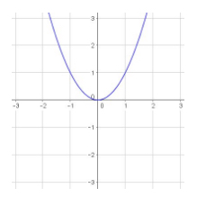
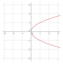
For an equation to qualify as a function, it must have only one output value for each input value. Graphically, an equation must pass the vertical line test; a vertical line must intersect the curve at only one point. This is best illustrated with an example:

$y = x^2$ is a function:

but $y = \pm\sqrt{x}$ is not a function:

Creating

Any situation that can be represented as an equation can also be written as a function in function notation. The variables upon which the output depends serve as the input variables, the function acts on those variables and the output results.

Consider the following scenario: Company XYZ manufactures and distributes electronic tablets. The cost to manufacture each tablet depends on the product of the number of tablets and the cost to make each tablet, $\$150.00$, along with an added service fee of $\$55.00$. Each tablet is sold for $\$399.00$.

A function to determine the cost of production per tablet, the revenue per tablet, and the profit can be generated from the information given.

Call the cost function, $c(x)$, where $x$ represents the number of tablets. It depends upon the product of number of tablets, $x$, and the cost to make each tablet, $\$150.00$, plus the service cost of $\$55.00$:

\[c(x) = 150x + 55\]

Likewise, the revenue function, $r(y)$, depends upon the product of the number of tablets sold, $y$, and the price of each tablet:

\[r(y) = 399y\]

The profit function, $p(x)$, is the difference between the cost to make the tablets and the income generated from selling the tablets:

\[p(x, y) = r(y) - c(x) = (399y) - (150x + 55) = 399y - 150x - 55\]

Notice that the number of tablets made does not necessarily need to equal the number of tablets sold. In the case where both the number made and the number sold are known, the overall profit can be found. If only $x$ or $y$ is known, the function can be rearranged to solve for the other variable, and different scenarios can be tested, like “how many tablets must be sold in order for the company to breakeven,” for example.

Evaluating

Evaluating a function entails substituting each input variable with a particular value. Consider these examples:

$y = 3x - 2$ and $y = 2x^2 + x - 5$

Rewrite each equation in function notation:

$f(x) = 3x - 2$ and $g(x) = 2x^2 + x - 5$

Now that the functions are written in function notation, we can evaluate the function with any input value. Let’s evaluate both function when $x = -2$. To do so, rewrite the function to evaluate at the input value:

$f(-2) = 3(-2) - 2$ and $g(-2) = 2(-2)^2 + (-2) - 5$

Notice that we have simply replaced each input variable with the value for which we wish to evaluate. And, applying the rules of arithmetic:

$f(-2) = -6 - 2 = -8$ and $g(-2) = 2(4) - 2 - 5 = 1$

Function notation allows interesting input values. For example, we can evaluate $g(f(x))$. Doing so entails substituting the $f(x)$ function into each input variable present in $g(x)$:

\[g(f(x)) = 2(3x - 2)^2 + (3x - 2) - 5 = 2(9x^2 - 12x + 4) + 3x - 2 - 5 = 18x^2 - 24x + 8 + 3x - 2 - 5 = 18x^2 - 21x + 1\]

We can also evaluate $g(f(-1))$:

\[g(f(-1)) = 18(-1)^2 - 21(-1) + 1 = 18 + 21 + 1 = 40\]

Functions can also be combined through addition, subtraction, multiplication and division. We will look at addition as an example:

\[f(x) + g(x) = (3x - 2) + (2x^2 + x - 5) = 2x^2 + 4x - 7\]

Graphing

All functions can be easily graphed by generating a collection of input/output values in the form of coordinate points. However, this is not always the most efficient method, and in order to avoid spending an inordinate amount of time computing output values from input values, it is highly recommended to become familiar with the general forms of the functions you will encounter.

Linear functions relate an input to an output through a constant value and produce straight lines when graphed:

$y = mx$, where $m$ is a constant

Quadratic functions contain a variable raised to a second power and produce parabolas when graphed:

$y = ax^2$, where $a$ is a constant

Cubic functions contain a variable raised to the third power and produce S-shaped graphs, with one end increasing infinitely and the other end decreasing infinitely:

$y = ax^3$, where $a$ is a constant

Higher order even functions, $y = ax^4$, $y = ax^6$, etc., behave similarly to quadratic functions. Higher order odd functions, $y = ax^5$, $y = ax^7$, etc., behave similarly to cubic functions.

Absolute value functions graph as two rays intersecting at a vertex:

$y = a\vert{x}\vert$, where $a > 0$ produces a vertex as the minimum, and $a < 0$ produces a vertex as the maximum.

Exponential functions graph as an upward (or downward) sloping curve that changes by a particular proportion over a set interval. Logarithmic functions and exponential functions exhibit an inverse relationship. Consequently, logarithms exhibit graphs similar to exponentials, though reflected about the line of symmetry $y = x$. The general form of an exponential is $y = a^x$ and the logarithmic equivalent is $log_a y = x$.

Trigonometric functions produce periodic functions or functions that repeat themselves at regular intervals. The general forms of the trig. functions will be covered below.

Interpreting

Interpreting functions entails assessing the data presented and drawing conclusions from it. Consider the following function presented as a table, with its corresponding graph:

The data shows the velocity of a car from $0$ to $6.5$ seconds. A wealth of information can be deduced from the table and graph presented.

Right away it can be concluded that the data represents a function—it passes the vertical line test because every input shows a unique output.

It can also be concluded that the variables time and speed are directly related- as one increases, the other increases as well.

The domain of the function is each of the time measurements, and the range of the function is each of the speed measurements.

The vehicle starts from rest (velocity equals $0$), and the timer starts once the vehicle begins moving.

The function is best approximated by a linear equation.

A similar analysis can be performed for any function.