High School Algebra I Study Guide for the STAAR test

Describing and Graphing Linear Functions, Equations, and Inequalities

Twelve of the 54 questions on the STAAR test will assess these skills.

Representing and Solving

This section deals with writing, graphing, as well as solving linear functions, linear equations and inequalities. Have your calculator ready!

Finding the Slope

Recall that slope is the difference in the $y$-coordinates over the difference of the $x$-coordinates for two given points on a line or $m=\dfrac{y_1-y_2}{x_1-x_2}$.

The equation of a line in slope-intercept form is: $y=mx+b$, where $m$ = slope and $b = y$-intercept.
A line in point-slope form is $y-y_1=m(x-x_1)$ where $(x_1, y_1)$ is a given point on the line and $m$ = slope.
The standard form of a line, which will be discussed later, is $Ax + By = C$, where $A$, $B$, and $C$ are real numbers.
Vertical lines have no slope, and a horizontal line has zero for its slope.

Example 1:

Find the slope of the line represented by $2x-5y=6$.

Changing the line from standard form to slope-intercept form, we get:

\[2x-5y=6\] \[2x-5y-2x=6-2x\] \[\frac{-5y}{-5}=\frac{-2x+6}{-5}\] \[y=\frac{-2x}{-5}+\frac{6}{-5}\] \[y=\frac{2}{5}x-\frac{6}{5}\]

So, the slope is $\frac{2}{5}$.

Example 2:

Find the slope of this graph of a line:

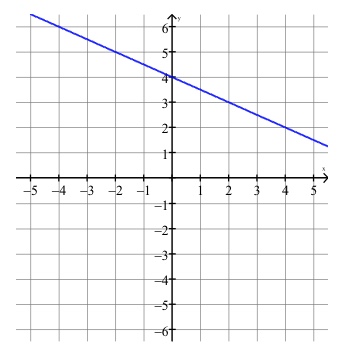
While you can choose any two points to find the slope, two convenient ones are the $y$-intercept of $(0, 4)$ and $(2, 3)$. So:

\[m=\dfrac{y_1-y_2}{x_1-x_2}=\dfrac{4-3}{0-2}=\dfrac{1}{-2}=-\dfrac{1}{2}\]

Finding the Rate of Change

The rate of change of a linear function is just the slope of the line formed by the graph of the function. In the context of problem-solving, the rate of change is a ratio or quotient of the change in one quantity versus another.

For example:

Suppose you can determine the distance you travel in a car over a period of time, and you record the distances traveled in the table below.

\[\begin{array}{|c|c|c|} \hline \text{time in hours} & \text{distance in miles} \\ \hline \text{1} & \text{42} \\ \hline \text{3} & \text{162} \\ \hline \text{4} & \text{222} \\ \hline \text{6} & \text{342} \\ \hline \end{array}\]

If the distance traveled over time forms a linear function, then find the rate of change and determine its meaning.

We can choose any two points since the slope is the same between any two points. Choosing the first two points, we get:

\[m=\frac{d_1-d_2}{t_1-t_2}=\frac{42-162}{1-3}=\frac{-120}{-2}=60\]

Since we found the difference in the distance traveled over the difference in time, our slope represents $60 \dfrac{\text{miles}}{\text{hours}}$ or $60 \text{ mph}$.

Another example:

You pour water into a barrel. The water level, $h$ , in inches of the barrel at time, $t$, in seconds, can be determined by the linear function $h=\frac{3}{7}t+4$. At what rate is the water level changing in the right cylinder?

The slope of the linear function is a quotient in change in the level of water over the change in time, which is $\frac{3}{7}$, so the water level is increasing at $\frac{3\;in.}{7 \;sec.}$.

Graphing Linear Functions

As you saw at the beginning of this category, a line in the form $y=mx+b$ can easily be graphed since we have slope and $y$-intercept.
Also, graphically, slope = $\frac{\text{rise}}{\text{run}}$.
You only need two points to graph a line.
The $x$-intercept, also called the zero, is a point where the graph of a line intersects the $x$-axis. If the equation is given for a line, it can be found by setting $y = 0$ and solving for $x$.
The $y$-intercept is a point where the line intersects the $y$-axis. It is the value of $b$ in slope-intercept form.

Example:

Find the $x$ and $y$ intercepts if the line is in standard form, $Ax + By=C$ when graphing the line.

Graph $y=\frac{2}{3}x+2$ and identify any intercepts.

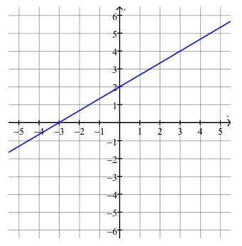
The slope and $y$-intercept are $m=\frac{2}{3}$ and $b=2$. Starting with the $y$-intercept of $2$, rise vertically up two units then run horizontally to the right three units to the point $(3, 4)$, which is also on the line. You can continue to do this but since you only need two points to graph a line, draw a line through the two points. The $x$-intercept is $-3$. It can also be confirmed by substituting $y = 0$ into our equation to get:

\[0=\frac{2}{3}x+2\] \[0-2=\frac{2}{3}x+2-2\] \[-2 \cdot \frac{3}{2} = \frac{3}{2} \cdot \frac{2}{3}x\] \[-3=x\]

Graphing Linear Inequalities

When graphing linear inequalities, you still graph the line, but you also shade the portion of the plane that is above or below the line to obtain the solution set. Consider these steps when working with these types of inequalities:

• For $\gt$ (dotted line) or $\ge$ (solid line) signs, shade above the line.
• For $\lt$ (dotted line) or $\le$ (solid line) signs, shade below the line.
• $x \lt a$ or $x \gt a$ is a vertical line where you shade to the left or the right of the line.
• $y \lt a$ or $y \gt a$ is a horizontal line where you shade below or above the line.
• Find the $x$ and $y$ intercepts if the line is in standard form, $Ax + By = C$ when graphing the line.
• Find the slope and $y$ intercept if the line is in the form $y=mx+b$.
• The region shaded on the plane is called the solution set or answer for the inequality.

For example:

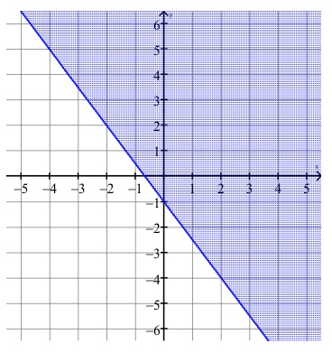
Shade the solution set for $y \ge =-\frac{3}{2}x-1$.

The line $y=-\frac{3}{2}x-1$ has a $y$-intercept of -1 and a slope of $-\frac{3}{2}$. The line is graphed in blue below. Since the inequality is greater than or equal to, shade above the line. The shaded region is the graph of the solution set.

Transforming the Parent Function

The parent function $f(x)=x$ is the diagonal line that passes thru the origin at a $45 ^\circ$ angle, as shown below.

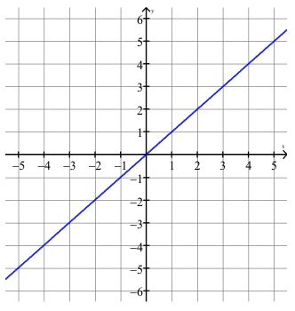
For the function $f(x)=x$, let $g(x)=a \cdot f(x-c)+d$. The graph of $g(x)$ is the graph of $f(x)$ where:

$a$ has a vertical stretch of $f$, if $a \gt 1$, and a vertical shrink if $0 \lt a \lt 1$. Also, if $a \lt 0$, then the graph of $f$ is reflected about the $x$-axis.
$c$ horizontally shifts the graph. If $c \gt 0$, the graph of $f$ shifts to the right, and it shifts to the left if $c \lt 0$.
$d$ vertically shifts the graph. If $d \gt 0$, the graph of $f$ shifts upward and shifts downward if $d \lt 0$.

Example:

State any transformations for $g(x)=-3(x+4)+2$ from the parent function, $y=x$.

Since $a$ is negative, the graph is reflected across the $x$-axis. The number $3$ is a vertical stretch by a factor of $3$, meaning each $y$ value for $y=x$ is multiplied by $3$. Next, $c = -4$, so the graph is shifted horizontally $4$ units to the right. Last, $d = 2$ so the graph is then shifted up by $2$ units.

Graphing Systems of Equations

When solving a system that has two linear equations, you can graph both of the lines on the coordinate plane and determine if they intersect. The point of intersection is the solution to the system since that point satisfies both linear equations.

Note: If the lines are parallel, they do not intersect, so there is no solution. If one line is a multiple of the other, they are the same line, so there are an infinite number of solutions.

For example:

Solve this system of equations graphically:
$y=2x-4$
$y=\frac{x}{2}+2$

The slope and $y$-intercept for the first line are $2$ and $-4$, respectively. It is graphed in blue below.

The slope and $y$-intercept for the second line are $\frac{1}{2}$ and $2$ respectively. It is graphed in red below.

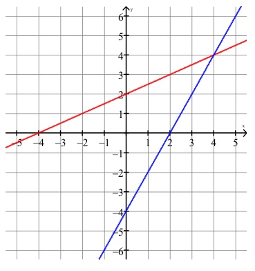
Examining the graphs of both lines, we can clearly see the point of intersection is at $(4, 4)$.

Graphing Systems of Linear Equations

Sometimes it is necessary to estimate the solution of two linear equations since the coordinates of their point of intersection will not be integer values.

For example:

The demand and supply functions for a stereo speaker are $y=60-5x$ and $y=25+3x$, respectively, where $x$ is the number of units sold in the hundreds and $y$ is the price in dollars. Estimate the break-even point (the point of intersection) for the number of units sold at a particular price.

Graphing both equations on a graphing calculator and determining a suitable graph to determine the point of intersection, we get the graphs below, where the first equation given is graphed in blue.

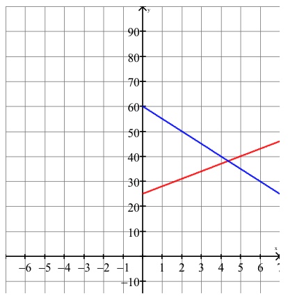
Estimating our solution, we see the point of intersection is approximately at $(4.3, 38)$ (the actual values are $(4.375, 38.125)$. So the number of speakers will be about $400$ and will sell for $\$38$.

Graphing Systems of Linear Inequalities

When graphing linear inequalities, you are generally looking for the common intersection that the inequalities have. Consider these steps when working with these types of inequalites:

For $\gt$ (dotted line) or $\ge$ (solid line) signs, shade above the line.
For $\lt$ (dotted line) or $\le$ (solid line) signs, shade below the line.
$x \lt a$ or $x \gt a$ is a vertical line where you shade to the left or the right of the line.
$y \lt a$ or $y \gt a$ is a horizontal line where you shade below or above the line.
Find the $x-$ and $y$-intercepts if the line is in standard form, $Ax + By = C$ when graphing the line.
Find the slope and $y$-intercept if the line is in the form $y=mx+b$.
The region shaded on the plane is called the solution set or answer for the inequality.

For example:

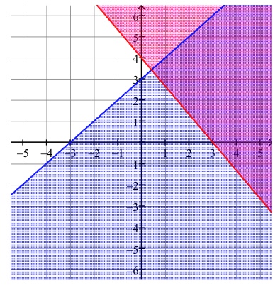
Shade the solution set for the following inequalities:

\[-x+y \le 3\] \[y \ge -\frac{4}{3}x+4\]

The line $-x+y=3$ has an $x$-intercept of $-3$ and a $y$-intercept of $3$. The line is graphed in blue below. Since the inequality is less than or equal to, shade below the line.

Then line $y \ge -\frac{4}{3}x+4$ has a $y$-intercept of $4$ and a slope of $-\frac{4}{3}$. The line is graphed in red below. Since the inequality is greater than or equal to, shade above the line.

The common shading between the two graphs is the solution set.

Forming and Evaluating Statistical Relationships

In this section, you will review how different methods, such as finding the correlation coefficient, determining a line of best fit for a given situation, and determining causation for a given situation, are used to find relationships for data that is provided in real-world situations.

Correlation

The correlation coefficient determines the measure of a set of data being linearly dependent. The correlation coefficient is $r$ on the graphing calculator where $-1 \le r \le 1$.

If $r = 1$ there is a strong positive linear relationship.
If $r = -1$, there is a strong negative linear relationship.
If $r = 0$, there is no linear relationship.
The closer $r$ is to zero, the weaker the linear relationship for the given set of data.

To find $r$ on a graphing calculator, follow these steps:

turn on the DiGnosticOn feature by typing the 2nd key, followed by the CATALOG key( or 0 key), then scroll down to DiGnosticOn and hit enter then hit enter again. The calculator returns done.
After putting your data set in the L1 and L2 lists, enter the STAT key, then scroll over to CALC, type in 8(LinReg) and hit enter. Then hit enter again and your line of best fit plus the correlation coefficient is displayed.

Example: What is the correlation coefficient for the following set?

\[\begin{array}{|c|c|c|} \hline \text{x} & \text{1} & \text{5} & \text{6} & \text{11} & \text{17} \\ \hline \text{y} & \text{28} & \text{38} & \text{42} & \text{58} & \text{74} \\ \hline \end{array}\]

Following the steps above to find $r$, we get $y=24.53+2.93x$ with $r=.997$, showing a very strong positive linear relationship between $x$ and $y$.

Association and Causation

Causation tells us that one event is the result of the occurrence another event, that is the change in variable directly causes changes in another variable in some experiment.

Association tells us that there is a relationship between two variables in an experiment, although there does not have to be a strong correlation or causation of them.

For example, is this true or false?

If a person studies more than his classmates, then that person will have a higher grade point average than his classmates.

While it can be shown that there could be a strong correlation and association in this instance, you cannot conclude that there will also be a causation, since there could be some classmates who study less but still have a higher grade point average.

As another example:

You make $\$13$ an hour working for a company. An increase in the number of hours you work in a given week has a direct effect on the increase in the amount of money you make for that week.

This is an example of a causation, since the increase in the number of hours you work causes your salary to increase.

But, what about this one?

The temperature is $31^\circ$, so it must be snowing.

While we can make an association from this statement, a below-freezing temperature alone does not cause it to snow. There are other factors involved, such as precipitation, to make it snow.

Best Fit

Using the method to find the correlation coefficient we can come up with a line of best fit in different situations to make predictions about future events.

For example:

The data below shows the number of gallons of water that are being poured into an empty hot tub that holds $500$ gallons of water. Write the line of best fit that shows how many gallons of water, $y$, are in the hot tub at time, $x$, in minutes and determine how long it will take to completely fill the hot tub.

\[\begin{array}{|c|c|c|} \hline \text{Minutes, x} & \text{1} & \text{4} & \text{10} & \text{12} & \text{17} \\ \hline \text{Gallons, y} & \text{17} & \text{77} & \text{165} & \text{218} & \text{300} \\ \hline \end{array}\]

Again, the steps for the line of best fit can be followed in the correlation coefficient section to get, $y=1.2+17.5x$, with a strong positive correlation. Setting $y = 500$, we can predict the amount of time it will take to fill the tub. Now:

\[500=1.2+17.5x\] \[500-1.2=17.5x\] \[498.8=17.5x\] \[28.5=x\]

(or about $28$ minutes and $30$ seconds)