Next Generation Quantitative Reasoning, Algebra, and Statistics Study Guide for the ACCUPLACER Test

Descriptive Statistics

Descriptive statistics is the method of visually representing data such that trends become apparent and we can draw conclusions. This includes measures of central tendency, like mean, median, and mode, but also measures of spread, like variance and standard deviation.

Data Display Types

Whereas functions do a good job of enabling particular phenomena to be represented graphically, when dealing with sets of data, it is often more elucidating to present the data in a different way.
Many different models are available for displaying data that enable immediate comparisons and conclusions to be made. Some of these models are covered here.

Histogram

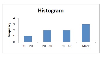
Histograms group data values into ranges and show the frequency at which each range occurs. Put another way, the height of the bar indicates how many data values fall within each range interval.

Box Plot

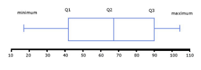
Box plots display the minimum, maximum, and quartiles of a data set. Quartiles will be discussed later in this section.

Scatterplot

Scatterplots show each data point on a coordinate plane.

Data Details

Quantifying the details of a data set facilitates the deduction of possible implications and conclusions. You will find a few ways of describing the details of a data set below.

Sample Set

A sample set is a collection of objects taken from a larger population in order to deduce potential characteristics of the population as a whole. The best sample sets are those that are randomly selected; however, this is not always an easy task.

Shape of a Sample Set

When represented graphically, a sample set, or distribution, can be described according to its skewness. ** Normally distributed** data sets exhibit a bell curve shape. Be sure not to misunderstand “normal” here as meaning “not unusual”. In statistics, “normal distribution” is the specific term used to refer to data sets with bell curve shapes.

Data that is skewed left is also described as negatively skewed and has its tail to the left and its peak to the right.

Data that is skewed right is also described as positively skewed and has its tail to the right and its peak to the left.

Measures of Center

The common measures of center: mean, median, mode,and midrange. These measures enable a set of data to be quantified. Consider the following set of data: \(\{1, \;1,\; 2,\; 3,\; 4,\; 5\}\)

The mean, also known as the average, is the sum of each data point divided by the total number of data points. In the example provided, the mean is:

\[\frac{1+1+2+3+4+5}{6} = \frac{16}{6} = 2.67\]

The median is the data point located in the middle of the data set (after it has been written in ascending or descending order). In the case of an even number of data points, the median is found by computing the average of the two middle values. So, in the example above, the median is:

\[\frac{2+3}{2} = 2.5\]

The mode is the data point that occurs most frequently. If there is no value that occurs most often, there is no mode.
In the example provided, the mode is \(1\).

The midrange is found by dividing the difference between the largest and smallest values in the set by \(2\). In this case, the midrange is:

\[\frac{5 - 1}{2} = 2\]

Spread of a Sample Set

The range, interquartile range, and standard deviation help quantify the spread of a sample set. Consider this sample set:

\[\{2, \;4,\; 4,\; 5, \;6, \;9, \;9, \;10\}\]

The range is the difference between the largest and smallest values in the set. For the sample provided, the range is \(10 - 2 = 8\).

The interquartile range is the difference between \(Q_1\) and \(Q_3\), where \(Q_1\) and \(Q_3\) provide the value corresponding to the \(25\)th and \(75\)th percentile, respectively.

The \(\bf{25}\)th percentile corresponds with the data point which is greater than \(25\)% of the other data points in the sample set.
The \(\bf{50}\)th percentile is the same as the median and is usually referred to by that name instead.

The quartiles can be found by dividing the sample set into four pieces. In cases where there is an even number of data points, just as the median is found by averaging the middle data points, the first quartile is found by averaging the middle values of the lower half, and the third quartile is found by averaging the middle values of the upper half.

In this case, the lower half middle values are \(4\) and \(4\), so \(Q_1 = 4\).

The upper half middle values are \(9\) and \(9\), so \(Q_3 = 9\).

The interquartile range is then \(9 - 4 = 5\).

The standard deviation quantifies the variation in the sample set. It is calculated by squaring the difference between each data point and the mean of the sample set, summing these squares and dividing the sum by the number of data points, then evaluating the square root of this value. For the data set provided, the mean is \(6.125\), so the standard deviation is (rounding a little)

\[\sqrt{\dfrac{ (2-6.125)^2 + (4-6.125)^2 \\ + (4-6.125)^2 + (5-6.125)^2 \\ + (6-6.125)^2 + (9-6.125)^2 \\ + (9-6.125)^2 + (10-6.125)^2}{10}}=2.9\]

Geometry for Pre-Algebra

Pre-algebraic concepts find ready application to geometry problems. Familiarity with the principles and rules of geometry helps us to use the techniques learned in pre-algebra and algebra to interpret and solve problems involving degree measures, distances, areas, and other concepts.

Perimeter

The perimeter is the distance around an object. For shapes that do not contain curved lines, the perimeter can be directly calculated by summing the side lengths.

Area

The area of a figure is a two-dimensional measurement of the amount of space contained within the figure’s edges. Familiarize yourself with the following area formulae:

Square: \(A = s^2\), where \(s\) is side length

Rectangle: \(A = lw\), where \(l\) is length and \(w\) is width

Trapezoid: \(A = \frac{1}{2}(b_1 + b_2)h\) where \(b_1\) and \(b_2\) are the bases (the two parallel sides) and \(h\) is the height

Triangle: \(A = \frac{1}{2}bh\), where \(b\) is the base and \(h\) is the height

Circle Area

The area of a circle is the product of the radius squared and pi. Stated algebraically:

\[A = \pi \cdot r^2\]

where \(\pi\) is approximately \(3.14\), and \(r\) is half of the diameter of the circle.

Circle Circumference

The circumference of a circle is the product of its diameter and pi. Stated algebraically:

\[C = \pi \cdot d\]

This formula is often written as \(C = 2\pi r\), where \(r\) is the radius.

Prism Volume

A prism is an object with flat sides that has the same shape on both ends, with the planes of those shapes parallel to one another and with parallel edges connecting the vertices of those end shapes. Consequently, the volume of a prism is calculated by multiplying the area of the end by the length of the prism.

Consider this example:

A prism of length \(10m\) is created from a triangle with a base of \(5m\) and a height of \(2m\).
What is the prism’s volume?

Recall that the area of a triangle is one-half the base times the height and the volume is the area of the triangle times the length of the prism. Stated algebraically:

\[V = (10\text{m}) \left( \frac{1}{2}(5\text{m})(2\text{m}) \right) = 50\;\text{m}^3\]

Volumes are three-dimensional measurements, so their units always have the form \(\text{units}^3\).

Geometry for Algebra I

The ability to analyze a scenario involving geometric concepts and principles, translate it into algebra, and then apply techniques to solve for unknown values is incredibly useful as you progress into upper-level math and science courses. Although geometry and algebra are treated as separate courses, there is a great deal of overlap between them and, in many cases, it will be difficult to decide whether you are working on a geometry or algebra problem. As such, it is critical that you expose yourself to as many problems of these types as you can, especially if you plan on going far in a STEM field.

Create Expressions

Math problems, especially real-world problems, very rarely present themselves in an obvious manner. It is up to us to translate a word problem into a collection of algebraic expressions or an algebraic equation. It is crucial that you develop this skill.

As is the case with everything, carefully reading or analyzing the situation or scenario is critical. This includes ensuring that details like unit conversions or cases with positive and negative solutions are considered and addressed.

Familiarity with the concepts of perimeter and area and their corresponding formulas facilitates an easy translation of word problems involving these topics.

Consider the following example: A circular pool is to have an area of 155 square meters. What must the pool’s diameter be?

To solve this, start with the formula for the area of a circle: \(A = \pi r^2\), where \(r\) is the radius, which is half the diameter. Substitute the known value and isolate \(r\):

\[155 = \pi r^2\] \[\frac{155}{\pi} = r^2\]

Square root both sides:

\[\sqrt{\frac{155}{\pi}} = r = 7.02\]

but this must be multiplied by \(2\) to find the diameter of \(14.04\) meters.

Consider this problem:

The volume of a particular cylinder is \(212\) cubic centimeters. If the height is twice the diameter, what is the radius?

Begin with the volume of a cylinder:

\[V = \pi r^2 \cdot h\]

It’s given that the height is twice the diameter, or \(h = 2d\), where the diameter is twice the radius, so \(h = 2d = 2(2r) = 4r\), which can be substituted into the original equation:

\[V = \pi r^2 \cdot 4r\]

Substitute the known value and solve for \(r\):

\[212 = 4\pi r^3\] \[\left( \frac{212}{4\pi} \right) ^{\frac{1}{3}} = r = 2.56\; \text{centimeters}\]

The Distance Formula

The distance formula is used to find the distance between any two points on a coordinate plane. Algebraically, the distance formula is stated as:

\[d = \sqrt{(x_2 - x_1)^2 + (y_2 - y_1)^2}\]

where \(d\) is the distance between the points and \((x_1, y_1)\; \text{and} \;(x_2, y_2)\) are the two points.

It is wise to learn the relationship between the distance formula together with the Pythagorean theorem, as they are essentially equivalent.

The Pythagorean Theorem

The Pythagorean theorem relates the side lengths of a right triangle to its hypotenuse. Stated algebraically, \(a^2 + b^2 = c^2\), where \(a\) and \(b\) are the side lengths and \(c\) is the length of the hypotenuse.

Transformations

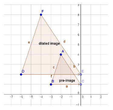
Familiarize yourself with the following geometric transformations: rotation, reflection, translation, and dilation.

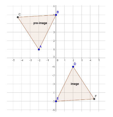
A rotation involves the movement of a figure about a fixed point. The rotated image is congruent to the original image. For example, \(180^\circ\) rotation about the origin of the following pre-image gives the image:

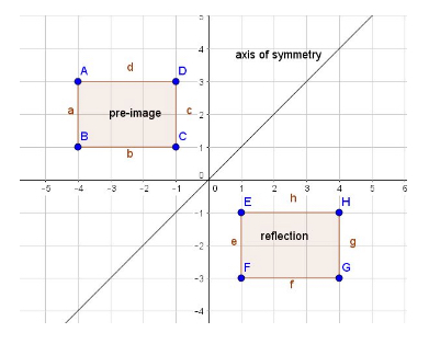
A reflection is a mapping of a collection of points across a line of symmetry. The reflection is congruent to the pre-image:

Translation entails moving the pre-image to another location. The translation is congruent to the pre-image:

A dilation is an increase or decrease in the size of an object. The dilated object is not congruent to the pre-image and the dilation will have a scale factor. Here we will use a scale factor of \(2\) (that is, for each point both the \(x\) and \(y\) coordinates of the pre-image will be multiplied by \(2\) to obtain the points of the image):