Next Generation Advanced Algebra and Functions Study Guide for the ACCUPLACER Test

Linear Applications and Graphs

Linear equations (and inequalities) find extensive applications in real world contexts. Developing the ability to assess a collection of variables and to produce an algebraic relationship or a graphical representation of a situation is invaluable not only for students pursuing a career in the STEM fields, but for anyone interested in presenting data or information to others.

Describing Relationships

Consider the relationship between the cost of an mp3 and the number of mp3s purchased. If each mp3 costs $0.99, a cost function can be generated showing the relationship between cost and number of mp3s purchased. Given that both the overall cost and the number of mp3s purchased are subject to change, we will use variables to represent each. Let $C$ represent the cost and $m$ represent the number of mp3s.

We know that each mp3 costs $\$0.99$, so we can produce a function that relates the cost and the number of mp3s through this constant price:

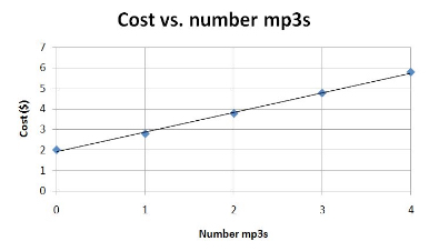
\[C = 0.99m\]

Notice that if no mp3s are purchased, the cost is $0$. If $10$ mp3s are purchased, the cost is $\$9.90$. What if, for example, there is a subscription fee of $\$2.00$ for using the mp3 service, but also a reduced cost for mp3s, $\$0.79$ instead of $\$0.99$. We can produce a new cost function:

\[C = 0.79m + 2.00\]

We have produced a linear equation that relates cost to number of mp3s purchased. We can translate this algebraic into a graph that looks like the following:

Now, consider a situation where in addition to mp3s, full albums can be bought for a price of $\$10.01$. We can use the cost function already established to generate a new cost function that includes the number of albums, $a$, purchased as well. Following the model already established, we can rewrite the cost function as:

\[C = 0.99m + 10.01a\]

This is a function in two variables, as a result, it requires $3$ dimensions to graph and will not be covered here.

Graphing

Graphing is the visual analog to the text-based algebraic function. Nearly every algebraic function can be generalized to a parent function. Develop familiarity with each of these parent functions in terms of their algebraic form as well as their graphic form. Doing so enables you to quickly deduce conclusions about the potential zeros and the end behavior of a function.

Linear Equations in Two Variables

Graphing a linear equation in two variables entails translating an equation like $y = 3x + 2$ into its corresponding picture:

2-linear-2-var..jpg

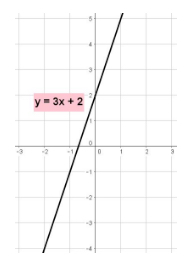
Any linear equation can be graphed by finding two points that satisfy the equation. One method for finding two points is to arbitrarily select a value for the $x$ variable, substitute it into the equation and solve for the $y$ variable.

For example, when $x = 0$, $y = 3x + 2$ gives $y = 3(0) + 2 = 2$, so $(0, 2)$ is a point on the line. When $x = 1$, $y = 3(1) + 2 = 5$, and $(1, 5)$ is another point on the line. Drawing a straight line through the plotted points gives the graph of the line $y = 3x + 2$.

Another method for graphing the line $y = 3x + 2$ is to notice that it is written in slope-intercept form, and explicitly provides both the slope and $y$-intercept of the line. The slope, in this case, is $3$, and the $y$-intercept is $2$ (recall that the $y$-intercept is the $y$-value at which the line passes through the $y$-axis).

To graph a line given in slope-intercept form, first plot the $y$-intercept $(0, y)$, then use the slope, to find the next point. In the case of the example already provided, with a slope of $\frac{3}{1}$, and $y$-intercept $(0, 2)$, the next point can be found by adding $3$ to the $y$-value, and adding $1$ to the $x$-value, to give $(1, 5)$.

The solution set to a linear equality is every point that lies along the line.

Linear Inequalities

Consider this linear inequality:

\[y > -x - 2\]

This should look very much to you like the equation of a line. And, for the most part, linear inequalities can be treated as linear equations. But, just as there is a caveat when solving linear inequalities, there is also a caveat when graphing them (in comparison with linear equalities).

The above inequality graphs as:

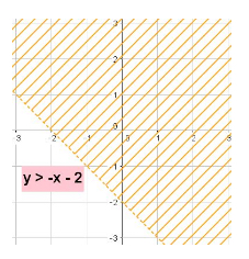
There are two details to notice in this graph:

One: the line formed by the equation $y = -x - 2$ is dashed.
Two: every point above the dotted line is shaded.

The $>$ in the inequality indicates that points lying along the line $y = -x - 2$ do not satisfy the condition of the inequality. Only the points lying immediately above the dashed line serve as solutions to the inequality, this is why the area above the line is shaded, the shading indicates the solution set.

Compare the inequality above with the inequality $y \le -x - 2$:

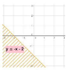
Notice that the inequality is now $\le$, the line is solid, and the area below the line is shaded. The equal sign in the inequality indicates that the points along the line $y = -x - 2$ satisfy the inequality and as a result are part of the solution set. Additionally, the shaded portion below the line indicates the points that belong to the solution set.

To gain an idea of what it means to be part of the solution set, let’s plug in $2$ values, one from the non-shaded area and one from the shaded area: $(0, 0)$ and $(-2, -1)$, respectively:

Trying $(0, 0)$: $0 \le 0 -2$, which becomes

$0 \le -2$, which is not a true statement, so the point $(0,0)$ is not part of the solution set, as can be seen from the graph.

Trying $(-2, -1)$: $-2 \le -(-1) - 2$, which becomes:

$-2 \le -1$, which is a true statement, so the point $(-2, -1)$ is part of the solution set, as can be seen from the graph.

Parallel and Perpendicular Lines

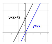
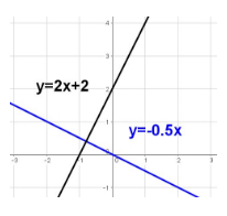
Algebraically, parallel lines are lines that share the same slope; perpendicular lines are lines that possess slopes that are negative reciprocals of each other (for example, the negative reciprocal of $\frac{3}{4}$ is $-\frac{4}{3}$).

Graphically, parallel lines never intersect.

Perpendicular lines intersect exactly once, and their intersection produces four congruent $90^\circ$ angles.

Systems of Equations

A system of equations can be any number of equations in any number of variables. As an example, we will consider three systems of two linear equations and show the distinct solution set possibilities.

The first case is a system of equations that share the same slope but have different axis intercepts:

$3x + y = -2$ and $3x + y = 1$, graphed here:

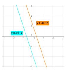
Equations that share the same slope but have different intercepts are parallel lines that never intersect. Because the solution set of a system of two linear equations is the point (or points) at which the lines intersect, a system of two parallel lines has no solution.

The second case is a system of linear equations that have different slopes that are not multiples of each other:

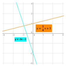
Linear equations that have different slopes that are not multiples of each other intersect at exactly one point. The point of intersection is the solution set of the system.

The third case is when one of the linear equations is a multiple of the other linear equation:

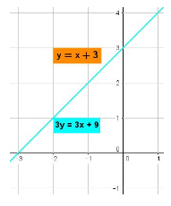
Notice that only one line color can be seen. This is because the other line color is underneath the blue color shown. Linear equations that are multiples of each other produce the same line when graphed, and as a result, the solution set is an infinite number of values corresponding to the infinite number of points that make up both lines.