Next Generation Quantitative Reasoning, Algebra, and Statistics Study Guide for the ACCUPLACER Test

Linear Applications and Graphs

Equations and graphs are different methods for representing the same thing. Just as an equation can be translated into its graphical representation, a graph can be represented with an equation. Consequently, when presented with a linear equation, you should be able to produce its corresponding graph, and when presented with the graph of a line, you should be able to generate its corresponding equation.

For example, provide the graph of the following linear equation:

\[-2y = 4x + 8\]

Begin by rewriting the equation in slope-intercept form by dividing both sides by \(-2\):

\[y = -2x - 4\]

The \(y\)-intercept is \((0, -4)\), and the slope, \(-2=\frac{-2}{1}\), gives a point that is \(2\) units below and \(1\) unit to the right of \((0, -4)\) as well as a point that is \(2\) units above and \(1\) unit to the left of \((0, -4)\):

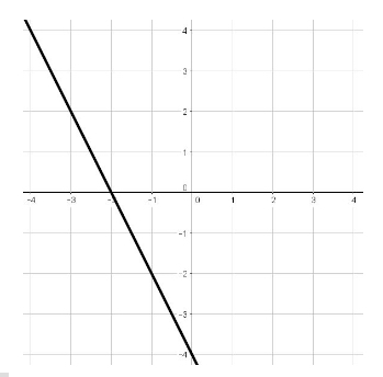
As another example going in the opposite direction, convert the following graph into a linear equation:

The line passes through the \(y\)-axis at \((0, 1)\), so the \(y\)-intercept is \(1\).
Notice that the line also passes through the point \((-3, 0)\)
The slope is then:

\[m = \frac{1 - 0}{0 - (-3)} = \frac{1}{3}\]

The equation in slope-intercept form is thus \(y = \frac{1}{3}x + 1\)

Use Linear Functions

A function relates an input variable to an output variable.
To qualify as a function, each input must correspond to a unique output.
Linear equations can be written as linear functions.

Consider this equation:

\[y = 3x + 4\]

In function notation this can be written as \(f(x) = 3x + 4\), which is read as “*\(f\) of \(x\) is equal to \(3x\) plus \(4\),” where \(x\) is the input variable and \(f(x)\) is the output variable.

Consider the following scenario:

Joyce’s rate of pay is a function of the number of hours she works. If she is paid \(\$13\) per hour, represent her rate of pay, \(P\), as a function of the number of hours she works, \(h\).

The input variable is the number of hours, \(h\), and the output value is her total pay, \(P\).
\(P\) is a function of \(h\): \(P(h)\), which is equal to her hourly wage times the number of hours worked; so \(P(h) = 13h\).

Graph Linear Equations in Two Variables

Linear equations in two variables come in a variety of forms: slope-intercept form, general form, and point-slope form. Each represents the line passing through \(2\) points on a coordinate or Cartesian plane.

Consider these two points: \((-1, -2)\) and \((2, 4)\)

The first is graphed as a point in Quadrant III with an \(x\)-value of \(-1\) and a \(y\)-value of \(-2\).
The second is graphed as a point in Quadrant I with an \(x\)-value of \(2\) and a \(y\)-value of \(4\).

The slope of the line connecting the two points is described by the formula:

\[m = \frac{y_2 - y_1}{x_2 - x_1}\]

where \(m\) represents the slope, and \((x_1, y_1)\) and \((x_2, y_2)\) represent the two points.

The \(y\)-intercept is the point at which the line passes through the \(y\)-axis.
The \(x\)-intercept is the point at which the line passes through the \(x\)-axis.

The slope-intercept form of a line explicitly provides both the slope and \(y\)-intercept of a line. It is generalized as the following:

\(y = mx + b\), where \(m\) is the slope, \(b\) is the \(y\)-intercept, and \((x, y)\) is any point along the line described by the equation.

The general form of a line is:

\[Ax + By + C = 0\]

where \(A\), \(B\), and \(C\) are numeric coefficients and \((x, y)\) is any point that satisfies the equation of the line.

The point-slope form of a line is stated generally as:

\[(y - y_1) = m(x - x_1)\]

where \(m\) is the slope and \((x_1, y_1)\) is a known point on the line, and \((x, y)\) represents any and every point on the line, satisfying its equation.

The slope of the line connecting the two points provided above is:

\[m = \frac{4 - (-2)}{2 - (-1)} = \frac{6}{3} = 2\]

The \(y\)-intercept can be determined by substituting a known point into the slope-intercept formula and solving for \(b\):

\[y = 2x + b\]

and substituting a known point

\[4 = 2(2) + b\] \[b = 0\]

Given any two points, exactly one line running through each can be constructed. When provided an equation for a line, two points on it can be found by substituting distinct values for \(x\) and determining their corresponding \(y\) values.

The pair \((x_1, y_1)\) and \((x_2, y_2)\) represent two points through which a line can be drawn.

Graph Linear Inequalities

Linear inequalities can be graphed in much the same way that linear equations can be graphed, with a few differences. It is useful to rearrange any linear inequality to its corresponding slope-intercept form. Once \(y\) is expressed in terms of \(x\), it is easy to decide which portion of the line (above or below) should be shaded, and given the inequality, it is easy to decide if the line should be dotted or bold.

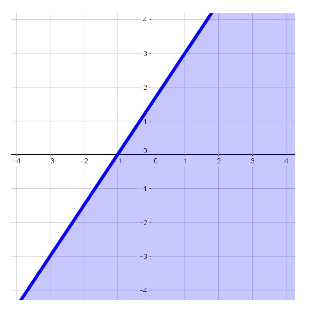
Consider the following example:

\[3x - 2y \ge -1\]

Begin by rearranging to slope-intercept form (solve for \(y\)):

\[-2y \ge -3x - 1\]

and dividing both sides by \(-2\), ensuring to switch the direction of the inequality because we are dividing by a negative value:

\[y \le \frac{3}{2}x + \frac{1}{2}\]

Right away the \(y\)-intercept can be found:

\[(0, \frac{1}{2})\]

Substituting \(x = 1\) enables another point to be found:

\[y \le \frac{3}{2}(1) + \frac{1}{2}\] \[y \le 2\]

The two points \((0, \frac{1}{2})\) and \((1, 2)\) lie along the bold line (\(\le\)), and the portion of the graph below the line is shaded to indicate the solution set:

Parallel and Perpendicular Lines

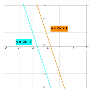
Parallel lines are those that have the same slope; they do not intersect when graphed.

Perpendicular lines are those that have negative reciprocal slopes; they intersect at one point when graphed, and they intersect to form right angles.

Graphing Systems of Equations

When graphed, a system of two linear equations will exhibit three distinct scenarios depending on the number of solutions to the system.

The three scenarios are as follows:

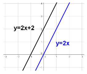
First case: The lines do not intersect and there is no solution to the system. This case arises from two lines that have the same slope but are not multiples of each other. Graphed:

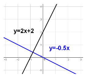
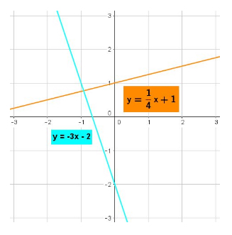
Second case: The lines intersect at one point and there is one solution to the system. This case arises from two lines that have a different slope.

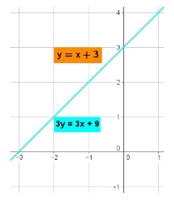
Third case: The lines intersect at every point and there are infinite solutions to the system. In this case, the two lines are really one and the same. This case arises from two lines that are multiples of each other. It graphs like this: