Formulas You’ll Need for the Accuplacer Next Generation Advanced Algebra and Functions Test

Navigating the ACCUPLACER Next Generation Advanced Algebra and Functions Test can seem like a daunting task, but with the right tools and preparation, you can confidently approach the exam. One of the most essential tools? A clear understanding of the formulas you’ll encounter and need to apply. Below, we’ll discuss some of the key formulas you should have at your fingertips during the test.

Linear Equations

Linear equations and inequalities serve as the backbone of algebra. These describe relationships that manifest as straight lines on a graph, making them paramount for grasping intricate mathematical notions. The ACCUPLACER underscores their importance, so let’s unpack them further.

The Slope-Intercept Form: y = mx + b

At the epicenter of linear equations is the slope-intercept form, represented as: y = mx + b

• Slope (m): The slope m is the rate of change of y relative to x. In layman’s terms, it gauges the steepness of the line. A positive slope implies the line ascends from left to right, while a negative one suggests a descent. A zero slope denotes a horizontal line, and an undefined slope is indicative of a vertical one.

• Y-Intercept (b): The y-intercept b signifies the juncture at which the line intersects the y-axis. Put differently, it’s the y value when x = 0.

Graphing Linear Equations

Sketching a line given its equation is an indispensable skill:

1. Start with the y-intercept: Begin by marking the point (0, b) on the graph, representing the y-intercept.

2. Utilize the slope to pinpoint another point: From the y-intercept, use the slope m as your compass. For instance, with a slope of 2, you’d rise by 2 units and traverse 1 unit to the right for the next point. If it’s -3, you’d descend 3 units and move 1 unit to the right.

3. Illustrate the line: Link the points to sketch your line.

Manipulating the Formula

It’s not merely about recognizing the formula, but also understanding its application in diverse scenarios:

• From Two Points: With two points but devoid of slope or y-intercept, you can employ them to ascertain the slope initially and then substitute one point into the equation to decipher b.

• From Slope and a Single Point: With the slope and a singular point, you can substitute them into the equation to solve for b.

Linear Inequalities

Adjacent to linear equations are linear inequalities, which, in lieu of the equal sign =, employ inequality symbols like \(>, <, \geq,\) or \(\leq\). These symbolize regions on the coordinate plane rather than mere lines. In graphing inequalities:

1. Graph the boundary line: This mirrors graphing a linear equation. For ‘greater than’ or ‘less than’, employ a dashed line, which indicates exclusion of the line from the solution. For ‘greater than or equal to’ or ‘less than or equal to’, utilize a solid line.

2. Shade the appropriate region: Opt for a test point, such as the origin (0,0), and substitute it into the inequality. If it satisfies the inequality, shade that side of the line; if not, shade the opposite side.

Linear Equation Formulas

Formula	Symbols	Comments
\(A\cdot x + B\cdot y = C\)	\(A, B, C = \text{any real number}\) \(y= \text{dependent variable}\) \(x = \text{independent variable}\)	Standard Form
\(y=m \cdot x + b\)	\(y = \text{dependent variable}\) \(m= \text{slope}\) \(x = \text{independent variable}\) \(b = y \text{-intercept}\)	Slope-Intercept Form. Try to convert linear equations to this format.
\(m = \dfrac{y_2 - y_1}{x_2 - x_1}\)	\(m = \text{slope}\) \(y_n = \text{dependent variable (point n)}\) \(x_n = \text{independent variable (point n)}\)	This is a rearranged version of the point-slope form.
\(y-y_1 = m(x-x_1)\)	\(y= \text{dependent variable}\) \(x = \text{independent variable}\) \(y_1 = y \text{ value of a point on the line}\) \(x_1 = x \text{ value of a point on the line}\) \(m = \text{slope}\)	Point-Slope form
\(x+a = b \Rightarrow x = b-a\) \(x-a = b \Rightarrow x = b+a\) \(x \cdot a = b \Rightarrow x = b \div a\) \(x \div a = b \Rightarrow x = b \cdot a\) \(x^a = b \Rightarrow x = \sqrt[a]{b}\) \(\sqrt[a]{x} = b \Rightarrow x = b^a\) \(a^x = b \Rightarrow x = \dfrac{\log b}{\log a}\)	\(a, b = \text{constants}\) \(x = \text{variable}\)

Quadratic Equations

Quadratic equations represent second-degree polynomials and are an integral part of algebra. Unlike linear equations, which produce straight lines when graphed, quadratics produce parabolic curves. Recognizing, solving, and graphing these equations are essential skills for the ACCUPLACER.

Understanding Quadratic Equations

A quadratic equation is generally expressed in the form: \(ax^2 + bx + c = 0\)

Where:

• a is the coefficient of \(x^2\) (and \(a \neq 0 \text{ because if it is, the equation becomes linear})\)

• b is the coefficient of x

• c is the constant term

The graph of a quadratic equation is called a parabola. Depending on the sign of the coefficient a, the parabola will open upwards (if a > 0) or downwards (if a < 0).

The Quadratic Formula

One of the most powerful tools for solving quadratic equations is the Quadratic Formula: \(x = \frac{-b \pm \sqrt{b^2 - 4ac}}{2a}\)

This formula provides the solutions (or roots) of the quadratic equation. Here’s a breakdown:

• \(\frac{-b}{2a}\) represents the axis of symmetry of the parabola, effectively giving you the x-coordinate of the vertex.

• \(\sqrt{b^2 - 4ac}\) is known as the discriminant. It helps in determining the nature of the roots:

• If \(b^2 - 4ac > 0\), the quadratic has two distinct real roots.

• If \(b^2 - 4ac = 0\), there is one real root (also known as a repeated or double root).

• If \(b^2 - 4ac < 0\), there are no real roots; instead, you have two complex conjugate roots.

Graphing and Interpreting Quadratics

Understanding the graph of a quadratic is crucial:

1. Vertex: This is the highest or lowest point on the graph, depending on the sign of a. The x-coordinate of the vertex can be found using \(-\frac{b}{2a}\), and the corresponding y-coordinate by substituting this x-value into the original equation.

2. Roots or Zeros: These are the x-values where the parabola intersects the x-axis. They can be found using the quadratic formula.

3. Axis of Symmetry: This is a vertical line passing through the vertex, dividing the parabola into two symmetrical halves. Its equation is \(x = -\frac{b}{2a}\).

4. Direction: Depending on the sign of a, the parabola will open upwards (positive) or downwards (negative).

Quadratic Equation Formulas

Formula	Symbols	Comments
\(x= \frac{-b \pm \sqrt{b^2-4ac}}{2a}\)	\(a,b = \text{constants}\) \(c = \text{constant (y-intercept)}\) \(x = \text{variable}\)	Quadratic Formula for equation in the form \(ax^2+bx+c=0\)
\((a \pm b)^2 = a^2 \pm 2ab + b^2\)	\(a,b = \text{constants or variables}\)	Square of a sum or difference
\(a^2-b^2 = (a+b)\cdot (a-b)\)	\(a,b = \text{constants or variables}\)	Difference of squares

Cubic Equations

Cubic equations, described by third-degree polynomials, advance our journey from quadratics in the realm of algebra. They depict a broader array of mathematical behaviors and set the stage for intricate algebraic challenges.

Definition of Cubic Equations

A cubic equation typically takes the form: \(ax^3 + bx^2 + cx + d = 0\)

Where:

• a is the coefficient of \(x^3\) and \(a \neq 0\) (if it’s zero, the polynomial reduces to either a quadratic or linear equation).

• b represents the coefficient of \(x^2\).

• c is tied to the coefficient of x.

• d is the standalone constant.

Roots of a Cubic

Every cubic equation possesses up to three real roots, but a minimum of one real root is guaranteed. The curve, representing the graph of a cubic function, might intersect the x-axis thrice or merely touch it. Depending on the equation’s specifics, roots can be real, repeated, or even complex.

Graphical Characteristics

Graphing a cubic equation reveals intriguing features:

1. End Behavior: The sign of a governs the curve’s trajectory. When a is positive, the curve ascends on the right. Conversely, a negative a sends the curve descending to the right.

2. Inflection Point: The curve possesses a point where it alters its concavity, switching between upward and downward curves.

3. Local Peaks and Valleys: These are the curve’s zeniths and nadirs, though they don’t necessarily denote the function’s absolute maximum or minimum.

Deciphering Cubic Equations

Solving cubic equations often presents a tougher challenge than quadratics. While advanced solutions like Cardano’s formula exist, they demand a deeper mathematical understanding compared to the quadratic formula. Typically, in foundational courses, learners leverage numerical strategies or factorization to derive approximate or specific solutions.

Cubic Equation Formulas

Formula	Symbols	Comments
\(a^3-b^3 = (a-b) \cdot (a^2+ab + b^2)\)	\(a,b = \text{constants or variables}\)	Difference of cubes
\(a^3+b^3 = (a+b) \cdot (a^2-ab + b^2)\)	\(a,b = \text{constants or variables}\)	Sum of cubes

Geometry Equations

Geometry, the mathematical study of shapes, sizes, properties of space, and dimensions, is another critical arena that students must conquer. Packed with formulas and rules, it demands both spatial intelligence and algebraic prowess to navigate effectively. From triangles to circles, and from area to volume, geometry equations provide tools to quantify and understand the space around us.

Essential 2D Shapes

1. Rectangle:

• Area: \(A = l \times w\) where \(l\) is the length and \(w\) is the width.

• Perimeter: \(P = 2l + 2w\)

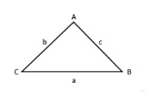
1. Triangle:

• Area: \(A = \frac{1}{2} b \times h\) where b is the base and h is the height.

• Pythagorean Theorem (for right triangles): \(a^2 + b^2 = c^2\), with c being the hypotenuse.

1. Circle:

• Area: \(A = \pi r^2\) where r is the radius.

• Circumference: \(C = 2\pi r\)

Key 3D Shapes

1. Cube:

   • Volume: \(V = s^3\) where s is the side length.

   • Surface Area: \(A = 6s^2\)

2. Sphere:

   • Volume: \(V = \frac{4}{3} \pi r^3\)

   • Surface Area: \(A = 4\pi r^2\)

3. Cylinder:

   • Volume: \(V = \pi r^2 h\) where h is the height.

   • Surface Area: \(A = 2\pi r(r + h)\)

Angles and Properties

Understanding various angle properties is fundamental in geometry:

1. Parallel Lines with a Transversal: Angles formed are either congruent (alternate interior, corresponding) or supplementary (same-side interior).

2. Triangles: The sum of internal angles is always \(180^\circ\).

3. Quadrilaterals: The sum of interior angles totals \(360^\circ\).

Coordinate Geometry

Merging algebra with geometry, coordinate geometry enables the study of geometric shapes using a coordinate system:

1. Distance between two points \((x_1, y_1)\) and \((x_2, y_2)\): \(D = \sqrt{(x_2-x_1)^2 + (y_2-y_1)^2}\)

2. Midpoint of a line segment joining \((x_1, y_1)\) and \((x_2, y_2)\): \(M = \left(\frac{x_1+x_2}{2}, \frac{y_1+y_2}{2}\right)\)

3. Slope of a line through \((x_1, y_1)\) and \((x_2, y_2)\): \(m = \frac{y_2-y_1}{x_2-x_1}\)

Geometry Formulas

Formula	Symbols	Comments
\(A = s^2\)	\(A = \text{area of a square}\) \(s = \text{side length}\)
\(A = l \cdot w\)	\(A = \text{area of a rectangle}\) \(l = \text{length}\) \(w = \text{width}\)
\(A = \dfrac{1}{2} b \cdot h\)	\(A = \text{area of a triangle}\) \(b= \text{base}\) \(h = \text{height}\)
\(A = \pi \cdot r^2\)	\(A = \text{area of a circle}\) \(r = \text{radius}\)
\(A = h \cdot \dfrac{b_1+b_2}{2}\)	\(A = \text{area of a trapezoid}\) \(b_n = \text{base }n\) \(h = \text{height}\)
\(C= 2 \pi r = \pi d\)	\(C = \text{perimeter of a circle}\) \(r = \text{radius}\) \(d = \text{diameter}\)
\(V = s^3\)	\(V = \text{volume of a cube}\) \(s = \text{side length}\)
\(V = l \cdot w \cdot h\)	\(V = \text{volume of a rectangular prism}\) \(l = \text{length}\) \(w = \text{width}\) \(h = \text{height}\)
\(V = \dfrac{4}{3} \pi r^3\)	\(V = \text{volume of a sphere}\) \(r = \text{radius}\)
\(V = \pi r^2 h\)	\(V = \text{volume of a cylinder}\) \(r = \text{radius of base}\) \(h = \text{height}\)
\(V = \dfrac{1}{3} \pi r^2 h\)	\(V = \text{volume of a cone}\) \(r = \text{radius}\) \(h = \text{height}\)
\(V = \dfrac{1}{3} l \cdot w \cdot h\)	\(V = \text{volume of a pyramid}\) \(l = \text{length}\) \(w = \text{width}\) \(h = \text{height}\)
\(d= \sqrt{\mathstrut (y_2 - y_1)^2 + (x_2-x_1)^2}\)	\(d = \text{distance between two points}\) \(y_n = y \text{ value at point n}\) \(x_n = x \text{ value at point n}\)
\(a^2 + b^ 2 = c^ 2\)	\(a,b = \text{legs of a right triangle}\) \(c = \text{hypotenuse of a right triangle}\)	Pythagorean theorem
\((x-h)^2 + (y-k)^2 = r^2\)	\((h,k) = \text{center of a circle}\) \(r = \text{radius}\)	Standard form of a circle
\(x^2 + y^2 + Ax + By + C = 0\)	\(x, y = \text{variables}\) \(A,B,C = \text{constants}\)	General form of a circle

Trigonometry Equations

Trigonometry, the branch of mathematics that studies relationships between side lengths and angles of triangles, plays a pivotal role in various scientific, engineering, and mathematical pursuits. Stemming from the Greek words “trigonon” (triangle) and “metron” (measure), it provides tools to bridge the gap between linear and angular measurements.

Basic Trigonometric Ratios

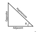
For a right-angled triangle, considering an angle \(\theta\):

1. Sine (sin):
   • Ratio of the length of the opposite side to the hypotenuse.
   • \[\sin(\theta) = \frac{\text{Opposite}}{\text{Hypotenuse}}\]
2. Cosine (cos):
   • Ratio of the length of the adjacent side to the hypotenuse.
   • \[\cos(\theta) = \frac{\text{Adjacent}}{\text{Hypotenuse}}\]
3. Tangent (tan):
   • Ratio of the length of the opposite side to the adjacent side.
   • \[\tan(\theta) = \frac{\text{Opposite}}{\text{Adjacent}} = \frac{\sin(\theta)}{\cos(\theta)}\]

Reciprocal Trigonometric Ratios

1. Cosecant (csc):
   • Reciprocal of sine
   • \[\csc(\theta) = \frac{1}{\sin(\theta)}\]
2. Secant (sec):
   • Reciprocal of cosine
   • \[\sec(\theta) = \frac{1}{\cos(\theta)}\]
3. Cotangent (cot):
   • Reciprocal of tangent
   • \[\cot(\theta) = \frac{1}{\tan(\theta)} = \frac{\cos(\theta)}{\sin(\theta)}\]

Key Trigonometric Identities

1. Pythagorean Identities:
   • \[\sin^2(\theta) + \cos^2(\theta) = 1\]
   • \[1 + \tan^2(\theta) = \sec^2(\theta)\]
   • \[1 + \cot^2(\theta) = \csc^2(\theta)\]
2. Angle Sum and Difference Formulas:
   • \[\sin(A \pm B) = \sin(A)\cos(B) \pm \cos(A)\sin(B)\]
   • \[\cos(A \pm B) = \cos(A)\cos(B) \mp \sin(A)\sin(B)\]
   • \[\tan(A + B) = \frac{\tan(A) + \tan(B)}{1 - \tan(A)\tan(B)}\]

Trigonometric Functions and Graphs

Understanding the behavior of trigonometric functions over the unit circle and their periodic nature is essential. The primary functions, sine, and cosine, repeat every \(2\pi\) radians or 360°. Their graphs showcase amplitude (height of the wave) and period (length before the wave pattern repeats).

Applications of Trigonometry

Beyond mere triangles, trigonometry finds applications in:

• Analyzing waveforms in electronics and sound.

• Astronomy for measuring distances and sizes of celestial objects.

• Engineering, especially in fields like civil and aeronautical engineering.

• Computer graphics and game design.

In essence, trigonometry offers tools to understand and quantify circular and harmonic motion, wave behavior, and the intrinsic relationship between angles and distances. Being conversant with its formulas and principles sets the groundwork for deeper dives into scientific and mathematical realms.

Trigonometry Formulas

Formula	Symbols	Comments
\(\sin^2 \theta + \cos^2 \theta = 1\)		Pythagorean Identity
\(\sin 2\theta = 2 \sin \theta \cdot \cos \theta\) \(\cos 2\theta = \cos^2 \theta - \sin^2 \theta = 2 \cos^2 \theta -1\) \(\tan 2\theta = \frac{2 \tan \theta}{1-\tan^2 \theta}\)		Double Angle formulas

Formulas with Diagrams

\[\sin \theta = \frac{\text{opposite}}{\text{hypotenuse}} = \frac{1}{\csc \theta} \\ \cos \theta = \frac{\text{adjacent}}{\text{hypotenuse}} = \frac{1}{\sec \theta} \\ \tan \theta = \frac{\sin \theta}{\cos \theta} =\frac{\text{opposite}}{\text{adjacent}} = \frac{1}{\cot \theta}\]

\[\dfrac{a}{\sin A} = \dfrac{b}{\sin B} = \dfrac{c}{\sin C} \\ a^2 = b^2 + c^2 -2bc \cos A \\ b^2 = a^2 + c^2 -2ac \cos B \\ c^2 = a^2 + b^2 -2ab \cos C\]

Wrapping Up Your ACCUPLACER Preparation

Embarking on the journey of the ACCUPLACER Next Generation Advanced Algebra and Functions Test is no small feat. From diving into the intricacies of algebra to navigating the expansive world of geometry, and scaling the peaks of trigonometry, there’s a plethora of content to master. However, with determination, the right tools, and strategic planning, success is well within your grasp.

Remember, understanding the foundational concepts is just the beginning. Practice, as they say, makes perfect. By leveraging our comprehensive ACCUPLACER practice tests, you can simulate the exam environment, identify areas of improvement, and solidify your knowledge. Our study guides offer in-depth explanations, ensuring that even the most complex topics become crystal clear. And for those quick revision sessions or last-minute prep, our ACCUPLACER flashcards serve as the perfect companion, distilling vast information into bite-sized, easily digestible chunks.

In conclusion, the ACCUPLACER might be challenging, but with dedication and the array of resources we offer, you are setting yourself up for success. Equip yourself, stay consistent, and remember: every equation, formula, and concept you conquer takes you one step closer to acing the test. All the best!